← Back to the plain-language case
The logistic-regression "odds ratios", including those in the abstract, appear to be log-odds coefficients
Psychol Med 2022;52(14):3289-3296 (published online 18 March 2021) · doi:10.1017/S0033291721000088 · PMC9693673
Summary
The paper reports two multivariable logistic regressions for clinically elevated hsCRP (⩾3 mg/L) and labels every estimate an odds ratio (OR). One of them is negative ("OR −4.39, 95% CI −7.04 to −1.97"), and six more have negative lower confidence limits (four distinct intervals; the age and gender intervals appear in both models). An odds ratio cannot be negative. Read as log-odds coefficients, the printed values hang together: every printed CI agrees with its printed p-value on significance at 0.05 (the interval excludes 0 exactly when p < 0.05), and the paper's own Table 1 counts reproduce the estimates closely (unadjusted log-odds 2.39 against the printed 2.44). Read as ORs, the two main-effect intervals in model 2 contradict their p-values. On the coefficient reading, the abstract's headline odds ratios are understated about 2.7- to 4.7-fold: "OR 2.44" corresponds to an OR of about 11.5 (95% CI 3.6 to 51.4), "OR 1.52" to about 4.6 and "OR 1.09" to about 3.0. The direction and significance of each finding are unchanged, but the effect sizes as printed are on the wrong scale, and read literally as ORs, the CI given for depression (0.27 to 2.01) includes 1 and would contradict the stated significance.
What the paper reports
Methods, "Statistical analysis":
To address the second hypothesis, two models of multivariable logistic regression were used. The first assessed how much risk comorbid depression and overweight contributed to the hsCRP levels ⩾3 mg/L relative to other participant groups, with age and gender as covariates. The second assessed how much risk depression and overweight status (BMI ⩾ 25) separately contributed to hsCRP levels ⩾3 mg/L, with age and gender as covariates.
Results, "High sensitivity C-Reactive Protein", first logistic paragraph (model 1):
Overweight patients with depression were at a significantly increased risk of having hsCRP ⩾3 mg/L [OR 2.44, 95% confidence interval (CI) 1.28 to 3.94, p < 0.001], overweight controls did not have a significantly increased risk of hsCRP ⩾3 mg/L (OR 1.51, 95% CI −0.33 to 2.87, p = 0.13), normal-weight patients with depression did not have a significantly increased risk of hsCRP ⩾3 mg/L (OR 1.08, 95% CI −0.6 to 2.4, p = 0.28), while normal-weight controls were at a significantly decreased risk of hsCRP ⩾3 mg/L (OR −4.39, 95% CI −7.04 to −1.97, p < 0.001). Age and gender were not significantly associated with hsCRP ⩾3 mg/L [OR 0.01, 95% CI −0.04 to 0.06, p = 0.621, OR 0.61, 95% CI −0.19 to 1.47, p = 0.145, respectively].
Results, same section, second logistic paragraph (model 2):
Depression status was significantly associated with hsCRP ⩾3 mg/L (OR 1.09, 95% CI 0.27 to 2.01, p = 0.013) and overweight status was significantly associated with hsCRP ⩾3 mg/L (OR 1.52, 95% CI 0.7 to 2.41, p < 0.001). Age and gender were not significantly associated with hsCRP ⩾3 mg/L [OR 0.62, 95% CI −0.04 to 0.06, p = 0.647, OR 0.01, 95% CI −0.19 to 1.47, p = 0.137, respectively].
Abstract, "Results":
Multivariable logistic regression showed that comorbid depression and overweight significantly increased the risk of clinically elevated hsCRP levels ⩾3 mg/L (OR 2.44, 1.28–3.94). In a separate multivariable logistic regression model, overweight status contributed most to the risk of having hsCRP levels ⩾3 mg/L (OR 1.52, 0.7–2.41), while depression also contributed a significant risk (OR 1.09, 0.27–2).
Table 1, row "hsCRP ⩾3 mg/L (%)". The columns are overweight & depressed (N = 69), overweight control (N = 35), normal weight & depressed (N = 55), normal weight control (N = 57), statistic, p:
hsCRP ⩾3 mg/L (%) | 26 (37.7%) | 5 (14.3%) | 6 (10.9%) | 3 (5.3%) | x2 = 25.96 | <0.001
The conclusions that rest on these models. Abstract, "Conclusion":
Comorbid depression and overweight status are associated with increased hsCRP, and the coexistence of these conditions amplified the risk of clinically elevated hsCRP levels. Overweight status contributed most to the risk of clinically elevated hsCRP levels, but depression also contributed to a significant risk.
Discussion, first paragraph:
Of clinical relevance, overweight patients with depression had the highest risk for hsCRP levels ⩾3 mg/L, indicating clinically elevated peripheral inflammation.
What the paper's own numbers show
Method. In logistic regression a coefficient β is a log odds ratio, and the odds ratio is exp(β). An OR must be positive and its null is 1, while a coefficient can take any sign and its null is 0. I made three checks:
- Sign. I checked each printed estimate and CI limit for values ⩽ 0, which no OR can take.
- CI against p-value. I took each printed CI as a 95% Wald interval and back-calculated the two-sided p-value it implies under two readings: as a coefficient (null 0) and as an OR (null 1, computed on the log scale). I also checked, more simply, whether each interval excludes the null exactly when the printed p is below 0.05. The printed intervals are not symmetric about their estimates, and most look like profile-likelihood intervals (see check 3), so a Wald back-calculation from them is only approximate. The significance check does not depend on that assumption.
- Refit from Table 1. I refitted both models without the age and gender covariates, using only the grouped counts in Table 1 (40 cases with hsCRP ⩾3 mg/L among 216 participants). The paper's covariate-adjusted models need individual data, so the refits show the scale and approximate size of the estimates, not their exact values. I report both Wald and profile-likelihood intervals for the refits, because most printed intervals are asymmetric about their estimates in the way profile-likelihood intervals are (2.44 lies 1.16 above its lower limit of 1.28 and 1.50 below its upper limit of 3.94).
Every number below is printed by recompute.py.txt. Quoted passages keep the paper's minus signs (U+2212); elsewhere minus signs are typed as hyphens.
| Quantity | Location | Reported | Recomputed from the paper's numbers |
|---|---|---|---|
| hsCRP ⩾3 mg/L by group | Table 1 | 26/69, 5/35, 6/55, 3/57; χ² = 25.96, p < 0.001 | 37.7%, 14.3%, 10.9%, 5.3%; Pearson χ² = 25.96, df 3, p = 9.7 × 10⁻⁶ (matches) |
| Overweight + depressed v. reference | Abstract; Results, model 1 | "OR 2.44 (1.28 to 3.94)", p < 0.001 | As a coefficient, the CI implies p = 0.0003 (matches p < 0.001); as an OR, it implies p = 0.002. Unadjusted refit: log-odds 2.39 (profile 1.26 to 3.87; Wald 1.13 to 3.65), p = 0.0002. Crude OR = (26/43)/(3/54) = 10.9. If the printed value is a coefficient, OR = exp(2.44) = 11.5 (3.6 to 51.4) |
| Overweight controls v. reference | Results, model 1 | "OR 1.51 (−0.33 to 2.87)", p = 0.13 | Negative lower limit is impossible for an OR. As a coefficient, the CI includes 0 (not significant, agreeing with p = 0.13), but a Wald back-calculation gives p = 0.064, about half the printed 0.13. Refit: log-odds 1.10 (profile -0.37 to 2.74; Wald -0.40 to 2.60), Wald p = 0.15. exp(printed) = 4.5 (0.72 to 17.6) |
| Normal-weight depressed v. reference | Results, model 1 | "OR 1.08 (−0.6 to 2.4)", p = 0.28 | Negative lower limit is impossible for an OR. As a coefficient, the CI includes 0 (not significant, agreeing with p = 0.28), but a Wald back-calculation gives p = 0.16, about half the printed 0.28. Refit: log-odds 0.79 (profile -0.60 to 2.39; Wald -0.65 to 2.23), Wald p = 0.28. exp(printed) = 2.9 (0.55 to 11.0) |
| "Normal-weight controls" | Results, model 1 | "OR −4.39 (−7.04 to −1.97)", p < 0.001 | Impossible as an OR. With four groups and an intercept, one group must be the reference and gets no coefficient of its own. Normal-weight controls are the reference implied by the other three contrasts. Their observed log-odds is ln(3/54) = -2.89, and the refit intercept is -2.89 (profile -4.30 to -1.89), so −4.39 is most consistent with the model intercept, which in the adjusted model refers to age 0 |
| Depression | Abstract; Results, model 2 | "OR 1.09 (0.27 to 2.01)", p = 0.013 | Read as an OR, the CI contains 1 and implies p = 0.87, contradicting p = 0.013. Read as a coefficient, it implies p = 0.014 (matches). Refit: log-odds 1.12 (profile 0.31 to 2.03), p = 0.010. exp(printed) = 3.0 (1.31 to 7.46) |
| Overweight | Abstract; Results, model 2 | "OR 1.52 (0.7 to 2.41)", p < 0.001 | Read as an OR, the CI contains 1 and implies p = 0.18, contradicting p < 0.001. Read as a coefficient, it implies p = 0.0005 (matches). Refit: log-odds 1.46 (profile 0.68 to 2.32), p = 0.00045. exp(printed) = 4.6 (2.01 to 11.1) |
| Age, gender | Results, model 1 | "OR 0.01 (−0.04 to 0.06)", p = 0.621; "OR 0.61 (−0.19 to 1.47)", p = 0.145 | Negative lower limits are impossible for ORs. As coefficients, implied p = 0.70 and 0.15. exp(printed) = 1.01 (0.96 to 1.06) per year and 1.84 (0.83 to 4.35) |
| Age, gender | Results, model 2 | "OR 0.62 (−0.04 to 0.06)", p = 0.647; "OR 0.01 (−0.19 to 1.47)", p = 0.137 | The age estimate 0.62 lies outside its own CI (-0.04 to 0.06). The two point estimates appear to be transposed relative to their CIs and to model 1 (0.01 with -0.04 to 0.06; 0.61 with -0.19 to 1.47). Both CIs include 0 and both p-values are above 0.05, so significance still agrees on the coefficient reading |
| Size of understatement | Abstract | 2.44, 1.52, 1.09 | exp(printed) / printed = 4.7×, 3.0×, 2.7× |
In the refit of model 1, the printed intervals and the profile-likelihood intervals line up closely: 1.28 to 3.94 against 1.26 to 3.87, -0.33 to 2.87 against -0.37 to 2.74, and -0.6 to 2.4 against -0.60 to 2.39. For overweight + depressed, depression and overweight, the printed intervals also share the refit's upward skew (for example 1.16 below and 1.50 above the estimate, against 1.13 and 1.48 in the refit). That pattern is what R's confint() gives for a glm fit on the coefficient scale. The Methods state that all analyses used R 4.0.0.
The Wald back-calculation is less exact. On the coefficient reading it matches the printed p for overweight + depressed (0.0003 v. < 0.001), "normal-weight controls" (0.0007 v. < 0.001), depression (0.014 v. 0.013), overweight (0.0005 v. < 0.001) and model 1 gender (0.15 v. 0.145), and is close to it for model 1 age (0.70 v. 0.621). For overweight controls (0.064 v. 0.13) and normal-weight depressed (0.16 v. 0.28) it gives about half the printed value, a gap a reader rerunning the script will see. In these two rows the printed limits are close to the refit's limits, but the printed estimates (1.51, 1.08) are higher than the refit estimates (1.10, 0.79). The printed estimates therefore sit nearer the upper limit (1.84 below and 1.36 above; 1.68 below and 1.32 above). The back-calculation divides the estimate by an SE taken from the interval width, so a larger estimate with the same width gives a larger z and a smaller p-value. The printed p-values for these two rows are close to the unadjusted refit Wald p-values (0.15 and 0.28). Because the printed intervals look like asymmetric profile intervals, a Wald back-calculation from them is only approximate, and these two rows cannot be resolved further without the model output. The gap is in size only: on the coefficient reading, no printed interval contradicts its printed p-value on significance at 0.05.
Figure
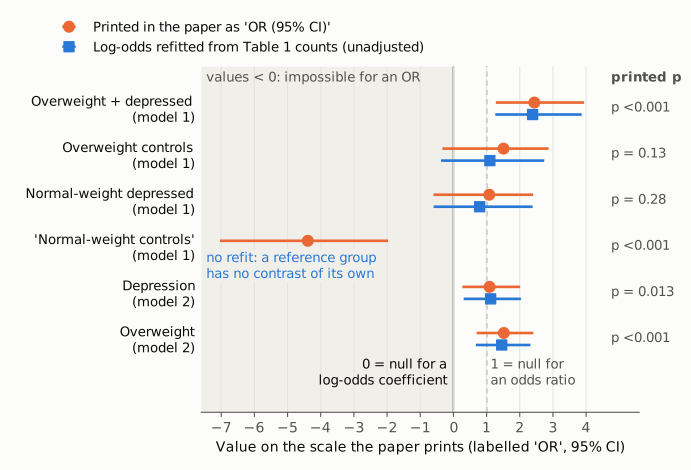
Each row is one group or main-effect estimate the paper prints with the label "OR"; the age and gender rows are not shown. Orange circles and lines are the printed estimate and 95% CI, on the linear scale on which they are printed. Blue squares and lines are log-odds coefficients refitted, without the age and gender covariates, from the hsCRP ⩾3 mg/L counts in Table 1, with profile-likelihood 95% intervals. The shaded region holds values below 0, which no odds ratio can take. The solid line at 0 is the null for a log-odds coefficient, and the dashed line at 1 is the null for an odds ratio. Whether each printed p-value (right) is below 0.05 matches whether its interval crosses 0, not whether it crosses 1. That is clearest for depression and overweight in model 2, whose intervals cross 1 but are reported as significant. The row labelled "normal-weight controls" has no blue refit because the reference group of a categorical predictor has no contrast of its own.
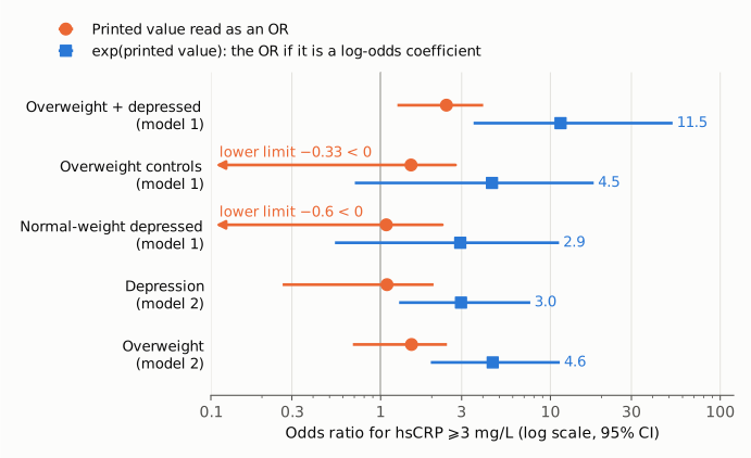
The same estimates on a log odds-ratio axis. Orange is the printed value taken literally as an OR. Lower limits below 0 cannot be placed on this axis and are drawn as arrows. Blue is exp(printed value), the odds ratio implied if the printed numbers are coefficients, labelled with its point estimate. The intercept-like "normal-weight controls" row is omitted because its printed value is negative. The age and gender rows of both models are not shown either.
Why it matters
The three figures in the abstract are the paper's quantitative answer to its second aim, "what extent overweight status and depression status contributed to clinically elevated hsCRP levels". As printed, they suggest modest associations: odds roughly 2.4, 1.5 and 1.1 times higher. If they are coefficients, the implied odds ratios are about 11.5, 4.6 and 3.0, a 2.7- to 4.7-fold difference. A reader citing these ORs, or pooling them in a meta-analysis, would carry the wrong magnitude. Read literally as ORs, the printed intervals also contradict the paper's own significance statements: the depression interval (0.27 to 2.01) and the overweight interval (0.7 to 2.41) both include 1. A reader who takes the label at face value could therefore conclude that neither main effect is significant, which is the opposite of what the abstract states.
The qualitative conclusions do not depend on the scale. Overweight-and-depressed participants have the highest odds, overweight contributes more than depression, and both are significant in model 2. Those orderings and significance calls are the same on either scale, and the Table 1 refits support them. The second-paragraph age and gender estimates are a separate, smaller transcription problem.
Explanations considered
- Conversion or typesetting artefact (lost or added minus signs). This does not account for the numbers. The evidence check found the same values, with true minus signs (U+2212), in the publisher's HTML and PDF on Cambridge Core and in the PMC and Europe PMC XML. Removing the signs would not help either: an OR of 4.39 would mean increased risk, while the text says normal-weight controls were at "significantly decreased risk".
- The printed values are ORs and only the negative ones are typos. This does not account for them. The positive-only intervals for depression (0.27 to 2.01) and overweight (0.7 to 2.41) would then contain 1 and imply p = 0.87 and p = 0.18, not the printed p = 0.013 and p < 0.001. Separately, the unadjusted crude OR for overweight-depressed v. normal-weight controls is 10.9, far from 2.44.
- The values are coefficients, correctly computed, and labelled "OR" in error. This accounts for everything checked. On the coefficient reading, every printed CI agrees with its printed p-value on significance at 0.05. Of the eight rows that are not transposed, a Wald back-calculation also matches the printed p-value closely for five and is close to it for a sixth, model 1 age (0.70 v. 0.621). It is about a factor of 2 low for overweight controls (0.064 v. 0.13) and normal-weight depressed (0.16 v. 0.28), whose printed p-values are instead close to the unadjusted refit Wald p-values (0.15 and 0.28). Since the printed intervals look like asymmetric profile intervals, the back-calculation is only approximate, and this gap does not point to a different scale: on the OR reading those two rows have impossible negative limits. The unadjusted refits from Table 1 give 2.39, 1.10, 0.79, 1.12 and 1.46 against the printed 2.44, 1.51, 1.08, 1.09 and 1.52, and their profile intervals closely match the printed intervals. The covariates would be expected to shift the estimates somewhat (age and gender differ between groups, Table 1), so small differences are expected.
- The "−4.39" is a genuine group contrast. Unlikely. With an intercept, only three of the four groups can have coefficients, and the three positive coefficients are the contrasts against normal-weight controls. −4.39 fits an intercept: the unadjusted intercept is -2.89, and an adjusted intercept refers to age 0, so a more negative value is expected. Its exact meaning cannot be confirmed without the model output.
- The supplement holds the correct output. It does not. The only supplementary file contains a non-smoker version of Table 1 and a consortium member list, with no regression output.
Status
As of 2026-10-23:
- Version of record. Checked on Cambridge Core (HTML and PDF, S0033291721000088a.pdf) and in the PMC and Europe PMC full-text XML. All four sources carry the same values, including the negative "OR" and the negative limits, so the problem is in the version of record and is not introduced by conversion.
- Supplement. The only supplementary file is S0033291721000088sup001.docx. It holds Supplementary Table 1 (non-smokers: hsCRP ⩾3 mg/L in 23/58, 4/32, 5/44 and 3/51; χ² = 24.405) and the consortium list. It has no logistic-regression output, so it cannot settle whether the values are coefficients or ORs.
- Corrections and notices. No correction, erratum, expression of concern, retraction or comment was found. Crossref shows no
update-to/updated-byrelations. The Crossref Labs updates feed, which carries the Retraction Watch data, is empty. PMC and Europe PMC show no linked notices (Europe PMC record PMID 33731235, no comment/correction list), and the Cambridge Core page shows none either. - Repository copy. The Cardiff ORCA repository has a record for the paper (orca.cardiff.ac.uk/id/eprint/138378). The site refused automated access (HTTP 403), so I did not check its full text or which version it holds. It could show whether the "OR" labels were already in the accepted manuscript.
- PubPeer. PubPeer refused direct access (HTTP 403), and a web search for the title with "PubPeer" found no PubPeer entry. So PubPeer was searched only indirectly.
- Sources. doi.org/10.1017/S0033291721000088; PMC9693673; Crossref REST API
api.crossref.org/works/10.1017/S0033291721000088; Europe PMC REST search.
Suggested correction
- State that the values reported in the logistic-regression paragraphs of the Results and in the abstract are log-odds coefficients (β), or replace them with odds ratios, exp(β), and their exponentiated CIs. If the printed values are the model coefficients, the abstract would read approximately:
- "OR 11.5, 95% CI 3.6–51.4" for comorbid depression and overweight;
- "OR 4.6, 2.0–11.1" for overweight;
- "OR 3.0, 1.3–7.5" for depression.
These values should be confirmed from the original model output. 2. In model 1, report the reference group explicitly (apparently normal-weight controls), and either drop the "−4.39" or label it as the intercept rather than as a risk estimate for normal-weight controls. 3. In the model 2 paragraph, check the age and gender estimates, which appear transposed (0.62 is printed with the interval -0.04 to 0.06). 4. Consider giving the full model output (coefficients, SEs, intercept and coding) in a table or supplement.