← Back to the plain-language case
Several adjusted odds ratios in the abstract have confidence intervals narrower than the data allow
Lancet Global Health (2025) · doi:10.1016/S2214-109X(25)00061-0 · PMC12208783
Summary
The Abstract, Results and Table 2 report adjusted odds ratios (aORs) for catastrophic health expenditure (CHE; 76 cases among 296 participants) of 2·0 (95% CI 1·9–2·1, p<0·0001) for the second vs first poverty quintile (60 participants each) and 9·7 (9·6–9·8) for subcounty hospitals vs health centres (69 vs 164 participants; 9·8 (9·7–9·9) in Table 2). For a 0/1 covariate held by this many participants, no model-based maximum-likelihood logistic regression can give a standard error below a floor set by the group sizes, and the standard errors implied by the two reported intervals are 11 and 52 times smaller than that floor; three further abstract aORs (female sex, education above secondary school, county hospital) are also below it, by smaller margins. With the standard error implied by the Table 1 counts, the second-quintile aOR becomes 2.0 (0.86–4.67, p = 0.11), close to the paper's own five-facility sensitivity estimate of 2.1 (0.70–6.1) in Supplementary Table 4. The second quintile is the only poverty quintile reported with significantly raised adjusted odds, and the abstract's conclusion that CHE is "driven by socioeconomic … inequalities" leans on it; the facility-level associations keep their direction and significance, but their stated precision is overstated about 50-fold.
What the paper reports
CHE was associated with being aged 30–44 years old (aOR 2·6, 95% CI 1·3–5·3, p=0·010), being female (1·8, 1·3–2·7, p=0·0021), having higher than secondary school education (1·6, 1·1–2·3, p=0·0083), being accompanied during health-care-seeking visits (3·2, 1·7–5·9, p<0·0001), belonging to the second poverty quintile (2·0, 1·9–2·1, p<0·0001), and seeking care from subcounty hospitals (9·7, 9·6–9·8, p<0·0001) and county hospitals (25·1, 15·7–40·2, p<0·0001).
Abstract, Findings
…belonging to the second poverty quintile (2·0, 1·9–2·1, p<0·0001), and seeking care from subcounty (9·7, 9·6–9·8, p<0·0001) and county hospitals (25·1, 15·7–40·2, p<0·0001; table 2).
Results, paragraph on CHE incidence
Table 2 ("Univariable and multivariable logistic regression of health and social factors associated with catastrophic health expenditure"). Its columns are the unadjusted OR (n=296), p, the adjusted OR (n=296) and p. Two of its rows read:
Second quintile | 1·4 (0·8–2·4) | 0·30 | 2·0 (1·9–2·1) | <0·0001
Subcounty hospital | 9·7 (8·4–11·1) | <0·0001 | 9·8 (9·7–9·9) | <0·0001
Table 2
Table 1 gives the counts behind these rows. The first quintile has 13 CHE and 47 no CHE, the second quintile 15 and 45, health centres 11 and 153, subcounty hospitals 27 and 42, and the county hospital 38 and 25.
How the paper uses these results:
…driven by socioeconomic and sex inequalities and impaired access to health care and social protection.
Abstract, Interpretation
Independent drivers of CHE included being female, poverty, being accompanied by a carer during health-care seeking, and seeking care at subcounty or county hospitals.
Research in context, Added value of this study
Our findings showed that poorer quintiles were more likely to incur CHE than the richest quintile, although the relationship across poverty quintiles did not always reach significance and appeared non-linear.
Discussion, paragraph 3
On the analysis, the paper says "Univariable and multivariable logistic regression models generated unadjusted and adjusted odds ratios", that "for the 21 participants without household asset data, multiple imputation with chained equations was also used to impute poverty scores", and "Data were analysed in STATA (version 15) and R (version 4)." (Methods, Statistical analysis). The paper does not describe a clustered, robust or otherwise non-standard variance estimator.
What the paper's own numbers show
Method. For a logistic regression coefficient on a 0/1 indicator held by n₁ of N participants, the model-based variance is the corresponding diagonal element of the inverse Fisher information. For any positive-definite matrix, a diagonal element of the inverse is at least the corresponding element of the inverse of any principal submatrix that contains it, so [I⁻¹]ⱼⱼ ≥ [(I_sub)⁻¹]ⱼⱼ, where I_sub is the intercept-and-indicator block of the same information matrix, evaluated at the full model's fitted values p. That block's inverse gives 1/S₁ + 1/S₀, where S₁ and S₀ sum p(1 − p) over participants with and without the indicator. Since p(1 − p) ≤ 1/4 always, SE ≥ √(4/n₁ + 4/(N − n₁)) for any covariate set and any fitted values. Pooling multiply imputed fits by Rubin's rules can only add variance. Separately, I derived each reported interval's implied SE, ln(upper/lower)/(2 × 1.96), including the full range allowed by rounding the printed limits to one decimal place. I computed crude ORs with Wald intervals from the Table 1 counts. All numbers come from recompute.py.txt.
| Quantity | Location | Reported | Recomputed from the paper's own numbers |
|---|---|---|---|
| aOR, second vs first poverty quintile | Abstract; Results; Table 2 | 2·0 (1·9–2·1), p<0·0001 | Implied SE 0.0255 (0.013–0.038 allowing for rounding), z = 27. Minimum possible SE with n₁ = 60: 0.289, which is 11× the implied SE and 7.5× the widest SE rounding allows. Narrowest possible 95% CI at aOR 2.0: 1.13–3.53 (p = 0.017) |
| Same, allowing for imputation of quintile in 21 participants | derived | — | If n₁ is anywhere from 39 to 81, the minimum SE is still 0.261, 10× the implied SE |
| Crude OR, second vs first quintile (15/60 vs 13/60) | Table 1 | Table 2 unadjusted: 1·4 (0·8–2·4), p=0·30 | 1.21 (0.52–2.81), SE 0.433, p = 0.67 (Fisher exact p = 0.83). Crude SE ÷ reported adjusted SE = 17 (11–34 allowing for rounding) |
| aOR 2.0 with the count-based SE | derived | — | 95% CI 0.86–4.67, p = 0.11 |
| Second quintile, same outcome and covariates with a five-level facility term | Supplementary Table 4 | 2.1 (0.70–6.1), p=0.099 | Implied SE 0.552, 22× the Table 2 SE. The interval includes 1 (the Wald p from this interval is 0.18) |
| aOR, subcounty hospital vs health centre | Abstract; Results | 9·7 (9·6–9·8), p<0·0001 | Implied SE 0.0053. Minimum possible SE with n₁ = 69: 0.275, 52× larger (35× the widest SE rounding allows). Narrowest possible CI at 9.7: 5.66–16.63 |
| aOR, subcounty hospital | Table 2 | 9·8 (9·7–9·9) | Differs from the Abstract and Results (9·7, 9·6–9·8). Same problem: minimum possible CI at 9.8 is 5.72–16.80 |
| Crude OR, subcounty vs health centre (27/69 vs 11/164) | Table 1 | Table 2 unadjusted: 9·7 (8·4–11·1) | 8.94 (4.10–19.50), SE 0.398, which is 76× the SE implied by the abstract's adjusted interval. aOR 9.7 with this SE: 4.4–21.2 |
| aOR, female | Abstract; Table 2 | 1·8 (1·3–2·7), p=0·0021 | Implied SE 0.186 (at most 0.201 allowing for rounding) vs minimum 0.236. Narrowest possible CI 1.13–2.86, p = 0.013 |
| aOR, above secondary education | Abstract; Table 2 | 1·6 (1·1–2·3), p=0·0083 | Implied SE 0.188 (at most 0.206) vs minimum 0.344. Narrowest possible CI 0.82–3.14, p = 0.17. Supplementary Table 4 gives 1.4 (0.50–4.2), p = 0.50 |
| aOR, county hospital | Abstract; Table 2 | 25·1 (15·7–40·2) | Implied SE 0.240 (at most 0.241) vs minimum 0.284. Narrowest possible CI 14.4–43.8. Still strongly significant |
| aOR, third quintile | Table 2 | 0·7 (0·6–0·9), p=0·0009 | Implied SE 0.103 (at most 0.139) vs minimum 0.293. Narrowest possible CI 0.39–1.24. Supplementary Table 4 gives 0.73 (0.22–2.4), p = 0.60 |
| aORs for age 30–44, accompanied, fourth and fifth quintile, NHIF | Abstract; Table 2 | e.g. 2·6 (1·3–5·3); 3·2 (1·7–5·9) | Consistent with the minimum (implied SE ≥ minimum) |
| Unadjusted secondary vs primary education (23/94 vs 42/163) | Table 1; Table 2 | 1·3 (1·2–1·5), p<0·0001 | Crude 0.93 (0.52–1.68), p = 0.82. Table 1 gives p = 0·90 for education |
| Unadjusted age 30–44 vs 18–29 (39/117 vs 14/103) | Table 1; Table 2 | 3·7 (2·9–4·6) | Crude 3.18 (1.61–6.29), SE 0.348 vs implied 0.118 |
| Unadjusted county vs health centre (38/63 vs 11/164) | Table 1; Table 2 | 24 (19·9–28·6) | Crude 21.1 (9.56–46.7), SE 0.405 vs implied 0.093 |
In the Abstract, 5 of the 7 adjusted associations have reported intervals narrower than any maximum-likelihood logistic fit to these data can produce. The violation is severe for the second quintile (11×) and subcounty hospital (52×). It is moderate for education above secondary school (1.8×). It is small for female sex (1.3×) and county hospital (1.2×). The bound is conservative: it assumes every fitted probability is 0.5, whereas the overall CHE rate is 26%. Realistic standard errors are larger, as the crude SEs and Supplementary Table 4 show.
The univariable column of Table 2 has the same pattern. Several of its intervals are much narrower than the crude counts give, and the secondary-education OR points the opposite way from the counts. That column appears unchanged in Supplementary Table 4, for example 3.7 (2.9–4.6), 1.3 (1.2–1.5) and 1.4 (0.76–2.4).
Figure
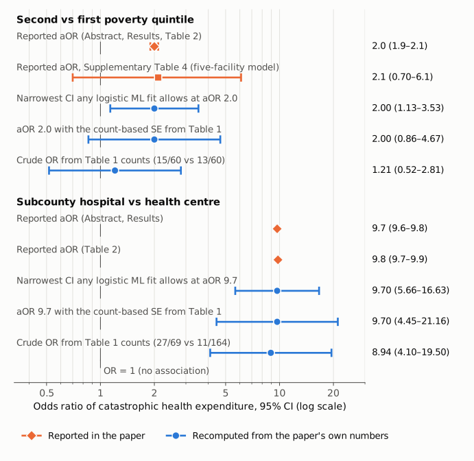
Figure 1. Odds ratios of catastrophic health expenditure with 95% CIs on a log scale. The thin vertical line marks OR = 1. Orange shows values the paper reports. For the second poverty quintile these are the main-model aOR 2.0 (1.9–2.1) from the Abstract, Results and Table 2 (diamond), and the same model with a five-level facility term from Supplementary Table 4 (square). For subcounty hospitals they are the Abstract and Results value 9.7 (9.6–9.8) and the Table 2 value 9.8 (9.7–9.9). Blue shows values recomputed from the paper's own numbers. The first blue row in each group is the narrowest interval any maximum-likelihood logistic fit could give at the reported point estimate. The second keeps the reported point estimate but uses the standard error of the crude log OR from the Table 1 counts. The third is the crude OR and Wald interval from those counts. The reported main-model intervals are hidden behind their markers. For the second quintile, the interval from the paper's own sensitivity model, the interval with the count-based SE (0.86–4.67) and the crude interval all include 1.
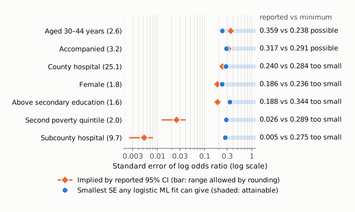
Figure 2. For each of the seven adjusted odds ratios in the Abstract (point estimate in brackets), the orange diamond is the standard error of the log OR implied by the reported 95% CI. Its bar is the range allowed by rounding the printed limits. The blue dot is the smallest standard error any maximum-likelihood logistic regression can give for that indicator, √(4/n₁ + 4/(296 − n₁)), with n₁ from Table 1. The shaded band to its right is the attainable range. Five of the seven reported intervals fall below this floor. The second-poverty-quintile and subcounty-hospital estimates are 11 and 52 times below it. The axis is logarithmic.
Why it matters
- The poverty finding. The second quintile is the only poverty quintile reported with significantly raised odds of CHE. The fourth and fifth quintile CIs include 1. The third quintile is reported as significantly lower, 0·7 (0·6–0·9), p=0·0009, but that interval is also narrower than the floor allows (narrowest possible CI 0.39–1.24), and Supplementary Table 4 gives 0.73 (0.22–2.4), p=0.60. With an attainable standard error, the second-quintile association is at most borderline: p = 0.017 at the theoretical minimum SE and p = 0.11 at the count-based SE. The paper's own five-facility sensitivity model gives 2.1 (0.70–6.1). The statements that CHE is "driven by socioeconomic … inequalities" (Abstract, Interpretation) and that poverty is an "independent driver" (Research in context) depend on this estimate. The Discussion already notes that the quintile relationship "did not always reach significance and appeared non-linear".
- Education and sex. At the minimum attainable SE, education above secondary school is no longer significant (narrowest CI 0.82–3.14). Supplementary Table 4 gives 1.4 (0.50–4.2), p = 0.50 for it, and 2.0 (0.95–4.0), p = 0.07 for female sex. The female aOR stays nominally significant at the bound (p = 0.013), but the bound is a floor, not an estimate.
- Facility level. The subcounty and county hospital associations keep their direction and remain highly significant with any plausible SE. Only their stated precision is wrong, by about 50-fold for subcounty hospitals.
- What stands. The CHE incidence (76/296, 26%), the cost breakdown, the NHIF coverage figures and the coping-strategy results do not depend on these intervals.
- Downstream use. A meta-analysis that takes 2.0 (1.9–2.1) or 9.7 (9.6–9.8) at face value would weight these estimates by inverse variance, that is, about 130 times (second quintile, 11.3²) and about 2,700 times (subcounty, 52.3²) more than even the theoretical floor on the standard error allows.
Explanations considered
- Rounding of the printed limits. Does not account for it. The widest interval consistent with "1·9–2·1" is 1.85–2.15, with SE 0.038, still 7.5 times below the floor. For "9·6–9·8" the factor is 35.
- A typo in one limit. Does not account for it. The second-quintile interval appears identically in the Abstract, Results and Table 2, and its p<0·0001 matches the interval (z ≈ 27). The subcounty value differs between Abstract (9·7, 9·6–9·8) and Table 2 (9·8, 9·7–9·9), but both are equally narrow. Four other adjusted intervals and several univariable intervals are also below the floor, so this is not one mistyped number.
- Covariate adjustment. Does not account for it. Adding covariates cannot push a model-based logistic-regression SE below √(4/n₁ + 4/(N − n₁)), as shown in the Method.
- Multiple imputation (21 participants without household asset data (Methods); 26 participants with missing income, expenditure or poverty data (Discussion)). Does not account for it. Rubin's total variance is at least the average within-imputation variance, and each of those obeys the bound. Even if imputation moved all 21 participants into or out of the second quintile, the bound would still be 0.261, 10 times the implied SE.
- Exact, penalised (Firth) or bootstrap intervals. None is mentioned in the paper, and for cells of this size (11 to 153 participants per cell in Table 1) such methods give intervals of similar width to the Wald interval, not 10–50 times narrower.
- A cluster-robust (sandwich) variance with facilities as clusters. This is the one standard estimator not bound by the inequality above. The paper does not mention it, and with five facilities, one of which forms the whole county-hospital level, such estimates are known to be unstable and too small. As a check, I computed the facility-clustered SE for the unadjusted three-level model from the facility counts in Supplementary Table 1b. These counts sum exactly to the Table 1 level totals. The result for county hospital (0.097, or 0.108 with the G/(G − 1) factor) is close to the 0.093 implied by Table 2. For subcounty hospital the result is 0.265–0.296, against 0.071 implied by Table 2. The Table 2 unadjusted ORs also differ from the crude ORs (9.7 vs 8.94; 24 vs 21.1). So this mechanism reproduces some of the reported intervals but not others. It cannot be confirmed without the data, and it would not make the reported intervals valid.
- A different sample or outcome in the model. Not supported. Table 2 states n=296 for both columns and the same 10% CHE outcome.
Status
- Version of record. The publisher's pages (thelancet.com, sciencedirect.com) and PDF were not reachable by automated access (HTTP 403/429). The open-access text deposited by the publisher was checked in the Europe PMC full-text XML for PMC12208783 (fetched 2026-10-23), the PMC article page and the local PMC archive copy. All carry 2·0 (1·9–2·1) and 9·7 (9·6–9·8) in the Abstract and Results, and 2·0 (1·9–2·1) and 9·8 (9·7–9·9) in Table 2. Every quotation above was checked verbatim against the archive copy. These are numbers in running text and table cells, not a rendering or conversion artefact.
- Supplements. Supplementary appendix 1 (mmc1.pdf, 2,538,411 bytes, md5 02ee6b399598cdef96ddbb2b8a1936e9, from the Europe PMC supplementary files) was read in full text. It contains Supplementary Table 4 (same 10% CHE outcome and covariates, with a five-level facility term), where the second quintile is 2.1 (0.70–6.1), p=0.099, and Supplementary Table 1b, which gives CHE by facility (5/85, 6/79, 12/38, 15/31, 38/63; these sum to the Table 1 level totals). It does not describe the variance estimator of the main model, and no individual-level data or code are provided. mmc2.pdf is a partnership declaration with no relevant data.
- Corrections. Crossref lists no update-to or updated-by relations, and PMC and Europe PMC list no correction, retraction or comment notice (checked 2026-10-23).
- PubPeer. pubpeer.com refused automated access (HTTP 403), and a web search could not be run in this session, so the absence of a PubPeer thread is not confirmed. Europe PMC's link services for PMID 40580995 list only a data citation and Altmetric, with no PubPeer link.
- As of 2026-10-23.
Suggested correction
- Re-estimate Table 2, both columns, with model-based maximum-likelihood standard errors, or state and justify the variance estimator used. With five facilities, a cluster-robust estimator is not appropriate without small-cluster corrections. Report the method in the Statistical analysis section.
- Replace the second-quintile, subcounty-hospital, female, above-secondary, county-hospital and third-quintile aOR intervals and p values in the Abstract, Results and Table 2. Also replace the univariable intervals that do not match the Table 1 counts.
- Reconcile the subcounty-hospital aOR between the Abstract and Results (9·7, 9·6–9·8) and Table 2 (9·8, 9·7–9·9).
- If the corrected second-quintile and above-secondary-education intervals include 1, revise the statements that poverty is an independent driver of CHE (Abstract Interpretation, Research in context, Discussion) and the abstract's list of associations accordingly.