← Back to the plain-language case
Two p-values for the recent-adversity estimates disagree with their own confidence intervals and forest plot
Psychol Med (2026) · doi:10.1017/S0033291726104632 · PMC13161794
Summary
The abstract and Results give two adjusted odds ratios for recent adversity from the joint-exposure model, which the paper names as its primary inferential model: aOR 1.91 (95% CI 1.47–2.49) without parental support, with p = .011, and aOR 1.76 (95% CI 1.17–2.65) with parental support, with p < .001. Recomputed from each printed aOR and CI, the p-values are about 1.5 × 10⁻⁶ and .0067. The paper's own forest plot for the same model prints "< .001" and "0.007", which agrees with the recomputation and not with the text. Both estimates stay significant at .05, so no conclusion is reversed. But the abstract presents the weaker of the two associations as the better established one.
What the paper reports
Abstract, Results:
Elevated odds from recent adversities (aOR = 1.91, 95% CI 1.47–2.49, p = .011) attenuated by parental support (aOR = 1.76, 95% CI 1.17–2.65, p < .001).
Results, "Temporal effects of adverse life events and parental support buffer", second paragraph (final model):
Compared to adolescents with no recent adversity and no parental support, those who experienced recent adversity but had no parental support had significantly higher PE odds (aOR = 1.91, 95% CI 1.47–2.49, p = .011). Among those with high parental support, recent adversity remained associated with elevated odds of PEs compared with those with no recent adversity and high parental support, although the magnitude of association was modestly attenuated (aOR = 1.76, 95% CI 1.17–2.65, p < .001).
Results, "Multivariable logistic regression modeling", first paragraph:
The joint exposure model demonstrated slightly improved explanatory value and is presented as the primary inferential model.
Methods, "Statistical analysis":
Adjusted odds ratios (aORs) with 95% confidence intervals were reported, and robust standard errors were applied.
Discussion, "Temporal effect of adversity and parental support buffer":
However, the magnitude of association was modestly attenuated in the presence of parental support (aOR 1.76 vs 1.91), suggesting partial buffering.
Forest plot of the joint-exposure model (an image, so not checked with the text tool; read from both the PMC and the publisher copies). The rows are "Adversities within 30 days and no parental support", printed as 1.92 (1.47 - 2.50), p < .001, and "Adversities within 30 days with parental support", printed as 1.76 (1.17 - 2.65), p 0.007.
What the paper's own numbers show
Method. For a logistic-regression aOR with a 95% Wald CI, SE(ln aOR) = (ln U − ln L) / (2 × 1.96), z = ln(aOR) / SE, and the two-sided p = 2 × (1 − Φ(|z|)). The paper used robust standard errors. The same robust SE gives both the CI and the p-value, so the check needs no other input. To allow for the two-decimal rounding of the CI, I also computed p for every CI whose bounds round to the printed ones. As a calibration, I applied the same method to eleven other estimates printed in the text. Their printed p-values agree with the recomputed ones to rounding, apart from one smaller side issue noted below. Every number below is printed by recompute.py.txt.
| Quantity | Location | Reported | Recomputed from the paper's own numbers |
|---|---|---|---|
| p, recent adversity without parental support | Abstract; Results | aOR 1.91 (1.47–2.49), p = .011 | SE 0.134, z = 4.81, p = 1.5 × 10⁻⁶. The range over CI rounding is 1.1 to 1.8 × 10⁻⁶. |
| p, recent adversity with parental support | Abstract; Results | aOR 1.76 (1.17–2.65), p < .001 | SE 0.209, z = 2.71, p = .0067. The range over CI rounding is .0062 to .0072. |
| Same two estimates in the joint-model forest plot | Forest plot image | 1.92 (1.47–2.50), p < .001; 1.76 (1.17–2.65), p = 0.007 | z = 4.82, p = 1.5 × 10⁻⁶; z = 2.71, p = .0067. Both agree with the plot. |
| CI that p = .011 would need, given aOR 1.91 | derived | 1.47–2.49 | SE 0.254 (1.89 times the printed CI's SE); 95% CI 1.16–3.15 |
| Widest CI that p < .001 allows, given aOR 1.76 | derived | 1.17–2.65 | SE below 0.172; 95% CI no wider than 1.26–2.46 |
| Recent adversity, main-effects model | Results | 1.86 (1.49–2.34), p < .001 | z = 5.39, p = 7 × 10⁻⁸. Consistent. |
| Undisclosed gender, SDQ ≤ 16 | Abstract; Results | 4.36 (1.50–12.66), p = .007 | p = .0068. Consistent. |
| Home safety, final model | Abstract; Results | 0.81 (0.66–0.99), p = .038 | p = .040 to .042. Consistent within CI rounding. |
| Financial hardship, final model | Results | 1.38 (1.07–1.79), p = .013 | p = .013 to .014. Consistent. |
| Low wellbeing, high school support | Results | 0.77 (0.61–0.98), p = .031 | p = .031 to .033. Consistent. |
| Side issue: high wellbeing, low school support | Results | 0.73 (0.57–0.95), p = .008 | p = .016 to .019. The forest plot prints 0.74 (0.57–0.96), p = .019. |
The log-scale midpoint of each printed CI matches its aOR: the geometric means are 1.913 and 1.761. So each aOR and its CI form a consistent pair. Only the p-values disagree with them, and they disagree in opposite directions. The printed p = .011 understates the evidence for the no-support estimate by a factor of about 7,000. The printed p < .001 overstates the evidence for the supported estimate: its own CI gives about .007. No CI that rounds to 1.17–2.65 can produce p < .001, because that p would need a lower bound of at least 1.26.
Figure
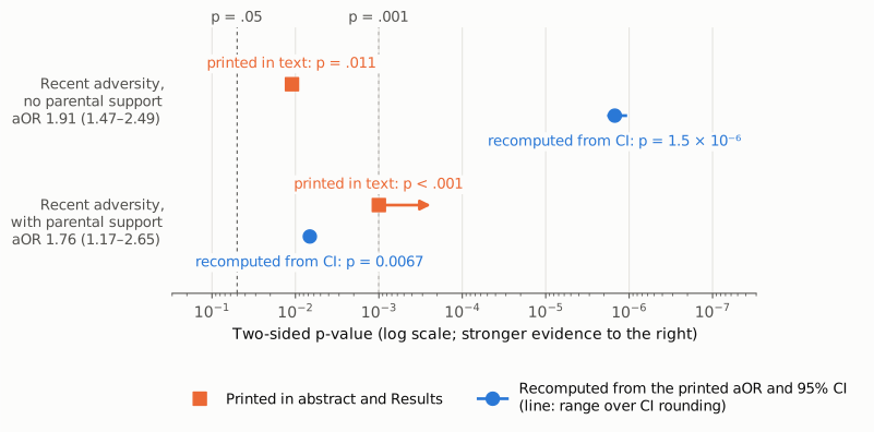
Figure 1. Two-sided p-values on a log scale, with stronger evidence to the right. Orange squares show the p-values printed in the abstract and Results. The arrow marks that "p < .001" is an upper bound. Blue circles show the p-values recomputed from the printed aOR and 95% CI with a log-scale Wald test. The short blue line is the range over all CIs that round to the printed bounds; for the second estimate it is narrower than the marker. Dashed lines mark p = .05 and p = .001. For the estimate without parental support, the printed .011 lies more than three orders of magnitude from the recomputed 1.5 × 10⁻⁶. For the estimate with parental support, the printed "< .001" lies on the wrong side of .001 from the recomputed .0067. The paper's own forest plot prints p < .001 and p = 0.007 for these two rows, in line with the blue values.
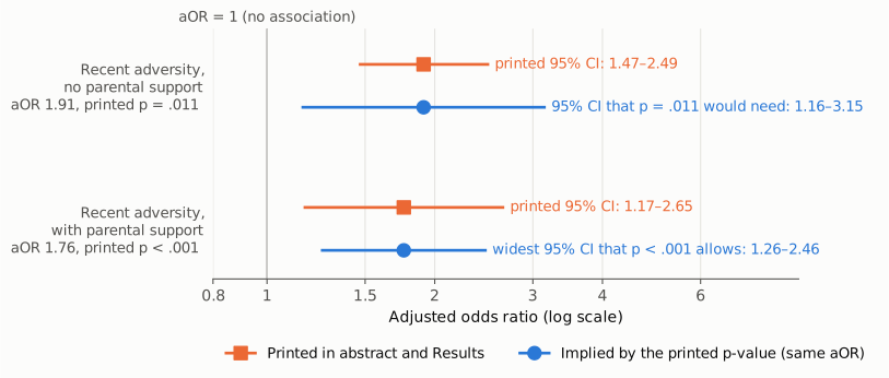
Figure 2. Adjusted odds ratios on a log scale. The thin vertical line is aOR = 1. Orange shows the printed aOR and 95% CI. Blue shows the 95% CI that the printed p-value would require, with the aOR held fixed. For p = .011, the interval around 1.91 would have to be 1.16–3.15, nearly twice as wide on the log scale as the printed 1.47–2.49. For p < .001, the interval around 1.76 could be no wider than 1.26–2.46, but the printed interval is 1.17–2.65. The printed CIs therefore cannot carry the printed p-values.
Why it matters
- The error is in the abstract and in the paper's primary model. The two estimates support the parental-support "buffer" message that the title ("Mitigating") and the Discussion highlight. A reader of the abstract alone sees p = .011 for the unbuffered association and p < .001 for the buffered one. That ordering is the reverse of what the paper's own intervals and forest plot show.
- No significance decision changes. Both associations are significant at .05 whichever p-values are used. The aORs and CIs, which carry the effect sizes, agree with each other, and they agree with the forest plot to within 0.01. The paper's conclusions that recent adversity is associated with PEs with or without parental support still hold. The no-support association is in fact better supported than the text states.
- The buffering claim rests on the point estimates, not on these p-values. The Discussion compares aOR 1.76 with 1.91. Neither p-value tests that difference. The two CIs overlap almost entirely, and the paper reports no test of the difference. The corrected p-values therefore neither add to nor take away from the buffering interpretation. They only remove an apparent sign that the supported group's estimate is the more firmly established one.
- Readers may reuse the numbers. Meta-analysts and readers who take p-values from abstracts would record the wrong strength of evidence for both estimates.
Explanations considered
- Rounding of the printed CI or aOR. Ruled out. Over every CI that rounds to 1.47–2.49, p ranges from 1.1 to 1.8 × 10⁻⁶. Over every CI that rounds to 1.17–2.65, p ranges from .0062 to .0072. Neither range comes near the printed value.
- Robust (sandwich) standard errors. Ruled out. The robust SE determines the CI as well as the p-value, so a Wald p from the printed robust CI already reflects it.
- Clustering by school or a t reference distribution. Ruled out. A t distribution with 3,700 df gives p = 1.5 × 10⁻⁶. Even with 39 df, as if the 40 schools were the units, p = 1.4 × 10⁻⁵. Any adjustment of this kind would also have widened the printed CI.
- A CI at another level. Ruled out. If 1.47–2.49 were a 90% CI, p would be 5 × 10⁻⁵. If it were a 99% CI, p would be even smaller. No conventional level yields .011.
- A Wald test on the odds-ratio scale, or a one-sided test. Ruled out. A linear-scale Wald test gives p = 4.7 × 10⁻⁴, and a one-sided log-scale test gives 7 × 10⁻⁷. Neither gives .011, and neither would explain the second estimate.
- The p-values swapped between the two estimates. Does not fully account for it. Exchanging them would make the first estimate correct ("< .001"), but the second would then read .011, while its CI gives .0067 and the forest plot prints 0.007.
- The value taken from the main-effects model. Ruled out. The main-effects estimate for recent adversity is 1.86 (1.49–2.34), printed and recomputed as p < .001.
- A text-conversion artifact. Ruled out. These values sit in running text, not in a table, with italic p and en-dash CIs. The publisher's HTML page, the Europe PMC JATS XML and the PMC archive all carry the same characters. A lost minus sign, a misread superscript or a shifted table cell cannot produce them.
- The text is right and the figure is wrong. Not supported. The forest-plot p-values agree with the CIs printed in both the text and the figure. The text p-values agree with neither.
- Side observations, not part of the main finding. (1) In both the PMC and the publisher copies, the image placed under the caption for Figure 1 ("main-effect" model) shows the joint-exposure estimates. The image under the caption for Figure 2 ("joint exposure" model) shows the main-effects estimates. The captions and images appear to be exchanged. (2) Several text aORs differ from the plotted values by 0.01, for example 1.91 vs 1.92 and 4.47 vs 4.48. (3) The forest plot lists a single reference row ("No adversities within 30 days and no parental support"), with "No adversities within 30 days with parental support" at 0.99 (0.83–1.19). The text, however, describes the 1.76 as relative to "no recent adversity and high parental support". If the 1.76 is against the common reference, the within-support contrast is 1.76 / 0.99 = 1.78; the conclusions do not change. (4) The text gives 0.73 (0.57–0.95), p = .008, for high wellbeing with low school support, but that CI implies p ≈ .016 to .019. The plotted 0.74 (0.57–0.96) is printed with p = .019 and recomputes to about .023.
Status
- Version of record. As of 2026-10-24, the publisher's page on Cambridge Core (reached through doi.org) carries the same values in the abstract and in the Results paragraph quoted above, as do the Europe PMC full-text XML and the PMC archive. Every quotation above was checked verbatim against the PMC-archived text with
src/show.py. The forest-plot values were read from both forest-plot images in the PMC copy, and the same values appear in the publisher's high-resolution image. - Supplements. The article has no supplementary material. The JATS XML has no supplementary-material element, and the Cambridge Core page data list none. The forest plots are the only other place where these estimates appear, and they resolve the discrepancy as described above.
- Corrections and comments. As of 2026-10-24 I found no correction, erratum, retraction or expression of concern.
src/known.pyreturns no Crossref updates, no PMC notices and no Europe PMC notices. The Crossref record has no update-to or updated-by field and an empty relation, and the Cambridge Core page data list empty corrections and retractions. The PubPeer API returned no record (HTTP 404) for the DOI, and a web search for the title together with "PubPeer" found no thread. - Sources. PMC article PMC13161794 and its two figure images; Europe PMC full-text XML; Cambridge Core article page via https://doi.org/10.1017/S0033291726104632; Crossref; PubPeer.
Suggested correction
In the abstract, replace
Elevated odds from recent adversities (aOR = 1.91, 95% CI 1.47–2.49, p = .011) attenuated by parental support (aOR = 1.76, 95% CI 1.17–2.65, p < .001).
with
Elevated odds from recent adversities (aOR = 1.91, 95% CI 1.47–2.49, p < .001) attenuated by parental support (aOR = 1.76, 95% CI 1.17–2.65, p = .007).
and make the same two changes in the second paragraph of the Results section "Temporal effects of adverse life events and parental support buffer". These are the values in the paper's own forest plot for the joint-exposure model. The authors may also wish to check:
- the p-value for high wellbeing with low school support (text p = .008; the CI implies about .016 to .019; the plot gives .019);
- the reference category stated for the 1.76 estimate;
- the 0.01 differences between the text and plotted aORs;
- the apparent exchange of the two forest-plot images between the Figure 1 and Figure 2 captions.