← Back to the plain-language case
The adjusted odds ratio for type 2 diabetes lies outside its own reported 95% CI
JAMA Netw Open (2025) · doi:10.1001/jamanetworkopen.2025.40818 · PMC12579343
Summary
The paper's one significant adjusted result is the association of polycystic ovarian morphology (PCOM) with non–insulin-dependent diabetes (NIDD). The abstract, the Results text and Table 3 all print it the same way: aOR 2.92, 95% CI 1.06–2.82, P = .02. The point estimate is larger than the upper confidence limit, so the estimate and the interval cannot both be right. The paper's own numbers allow two quite different repairs: an adjusted OR of about 1.73 if the interval is right, or an interval of about 1.06–8.04 if the estimate is right. Either way, readers cannot tell from the paper how large or how precise the key adjusted effect is. The direction and nominal significance hold under both readings.
What the paper reports
Abstract, Results:
Multivariate analysis confirmed the association of PCOM with non–insulin-dependent diabetes (aOR, 2.92; 95% CI, 1.06-2.82; P = .02).
Results, section "Logistic Regression Analysis":
The multivariate analysis indicated a significantly higher risk of NIDD in women with PCOM, with an aOR of 2.92 (95% CI, 1.06-2.82; P = .02).
Table 3 ("Logistic Regression Analysis of Chronic Morbidity and Mortality Among Women With PCOM"), NIDD row, under the column "aOR vs women without PCOM (95% CI)" and "P value":
NIDD | 2.92 (1.06-2.82) | .02
Table 3, footnote a:
All models were adjusted for age at enrollment; body mass index (calculated as weight in kilograms divided by height in meters squared); fasting insulin, total cholesterol, and triglyceride levels; and follow-up duration.
Table 2, NIDD row (PCOM, n = 189 | non-PCOM, n = 151 | P value):
NIDD | 45 (23.80) | 14 (9.27) | <.001
Methods, "Statistical Analysis":
P values presented in the logistic regression analysis are adjusted for multiple comparisons using the false discovery rate method. A post hoc Bonferroni correction was applied to the primary outcome (non–insulin-dependent diabetes [NIDD]) to confirm robustness of the finding.
Discussion, "Strengths and Limitations":
It could be claimed that the statistically significant finding in NIDD was due to multiple analyses being performed; however, even when adjusting for multiple comparisons using the Bonferroni correction, this outcome remained significant.
What the paper's own numbers show
Method. In a logistic regression the 95% Wald interval for an odds ratio is exp(b ± 1.96·SE). The estimate must therefore lie inside the interval and equal its geometric midpoint, √(lower × upper). Given any two of estimate, lower limit, upper limit and P, the other two follow. Profile-likelihood and other exact intervals are not exactly log-symmetric, but they still always contain the maximum-likelihood estimate. To check that the paper's intervals are of this kind, I applied the same test to all 27 estimated rows of Table 3. I also computed the crude odds ratio from the Table 2 counts. It is not an adjusted estimate and cannot replace one, but it shows which range is plausible. Every number below is printed by recompute.py.txt.
| Quantity | Location | Reported | Recomputed from the paper's own numbers |
|---|---|---|---|
| Is the NIDD aOR inside its CI? | Abstract; Results; Table 3 | 2.92 (1.06–2.82) | No. 2.92 exceeds the upper limit by 0.10. Rounding to 2 decimals leaves a gap of at least 0.09 |
| Geometric midpoint of the NIDD CI | Table 3 | estimate 2.92 | 1.73 |
| Reading A: CI 1.06–2.82 correct | Table 3 | aOR 2.92, P = .02 | aOR 1.73, SE(log OR) 0.250, z = 2.19, P = .028 (.027–.030 over the rounding range of both limits). Excess odds 73% instead of 192% |
| Reading B: aOR 2.92 and lower limit 1.06 correct | Table 3 | upper limit 2.82 | upper limit 8.04, SE 0.517, z = 2.07, P = .038 |
| Reading C: aOR 2.92 and upper limit 2.82 correct | Table 3 | lower limit 1.06 | lower limit 3.02, which is above the upper limit, so this reading is impossible |
| CI implied by aOR 2.92 with P = .02 | Table 3 | 1.06–2.82 | 1.18–7.20 (1.14–7.45 for P = .025) |
| Estimate implied by upper limit 2.82 with P = .02 | Table 3 | 2.92 | 1.76, with lower limit 1.09 |
| Crude NIDD OR, 45/189 vs 14/151 | Table 2 | 23.80% vs 9.27%, P < .001 | 23.81% vs 9.27%; OR 3.06 (Wald 95% CI 1.61–5.82); χ² = 12.37, P = .0004 |
| Other Table 3 rows: estimate ÷ CI midpoint | Table 3 | — | 0.91 to 1.33; 21 of 25 within 5%. The largest departures are rows with a printed lower limit of 0.01–0.02 |
| Other Table 3 rows: printed P vs Wald P from estimate and CI | Table 3 | — | median absolute difference 0.007 (maximum 0.035) |
| Hypothyroidism aOR (another row) | Table 3 | 0.55 (0.30–3.00), P = .052 | CI midpoint 0.95. If the estimate and lower limit are right, the upper limit is 1.01 with P = .053, matching the printed P |
| Time in study, mean difference | Table 2, footnote a | −1.42 (95% CI −6.25 to −2.22) | Interval does not contain −1.42. From the means and SDs, Welch 95% CI −2.28 to −0.56 |
| Age at death, mean difference | Table 2, footnote a; P in Table 2 and abstract | −16.58 (−35.77 to 2.60), P = .08 | From 54.25 (11.52), n = 7 vs 70.83 (13.64), n = 9: Welch CI −30.09 to −3.07, P = .020. The printed CI implies an SE of 8.94, against 6.30 from these SDs and counts |
| Age at follow-up, mean difference (control) | Table 2, footnote a | −5.96 (−7.86 to −4.06) | −5.96 (Welch −7.87 to −4.05): consistent |
The NIDD interval is the only one in Table 3 that excludes its own estimate. The other 25 rows sit on or near the line where estimate equals interval midpoint (Figure 2), so the paper's intervals behave as expected. The NIDD row is not.
The available evidence does not pick one reading. The crude OR (3.06) is close to 2.92, which favours Reading B. The printed P value, however, fits the printed interval better than the printed estimate. If it is a raw P, the interval alone implies P = .028, while the estimate with the lower limit implies P = .038. If it is FDR-adjusted, as the Methods state, the raw P behind it must be below .025, since adjustment can only raise a P value. Neither reading meets that exactly.
Figure
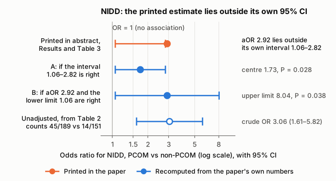
Figure 1. Odds ratio for non–insulin-dependent diabetes in women with vs without PCOM, on a log scale. The orange row is the adjusted estimate and 95% CI exactly as printed in the abstract, the Results text and Table 3: the dot (2.92) lies outside the bar (1.06–2.82). The blue rows are recomputed from the paper's own numbers. A keeps the printed interval and places the estimate at its geometric midpoint (1.73, P = .028). B keeps the printed estimate and lower limit and gives the log-symmetric upper limit (8.04, P = .038). The open circle is the unadjusted OR from the Table 2 counts (3.06, 1.61–5.82), shown for scale only. The thin vertical line marks OR = 1.
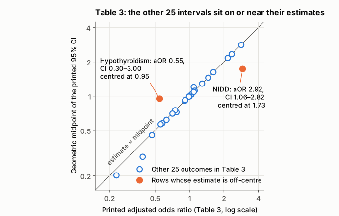
Figure 2. Each point is one outcome in Table 3. The x-axis is the printed aOR and the y-axis is the geometric midpoint of its printed 95% CI, both on log scales. For a standard logistic-regression interval the point lies on the diagonal. Twenty-five rows (open blue circles) lie on or near it; the largest departures, below the line at the lower left, are rows whose lower limits are printed as 0.01 or 0.02 and are therefore heavily rounded. The two orange points are off the line: NIDD (estimate 2.92, midpoint 1.73) and hypothyroidism (estimate 0.55, midpoint 0.95). This shows that the NIDD interval is the exception in a table whose intervals are otherwise centred on their estimates.
Why it matters
- It is the paper's key adjusted result, and it is printed in the abstract. The Key Points and the Conclusions describe PCOM as associated with an increased risk of type 2 diabetes. After adjustment for age, BMI, fasting insulin, lipids and follow-up, the only support for this is the NIDD aOR. Readers citing "aOR 2.92 (1.06–2.82)" are citing a pair of numbers that cannot both be correct.
- The size and precision of the effect cannot be recovered. Under Reading A, the adjusted excess odds are about 73% (OR 1.73), well under half the printed 192%. Under Reading B, the estimate stands but the interval runs from about 1 to 8, so the data are far less precise than the printed interval suggests. These two readings would lead to different conclusions in a meta-analysis, in a risk-communication setting or in a sample-size calculation.
- The conclusion that the association exists is not overturned. In both readings the lower limit stays at about 1.06 and the unadjusted P stays below .05, and the crude counts (23.8% vs 9.3%) point the same way. The error concerns how large and how precise the adjusted association is, not whether there is one.
- The robustness claim cannot be checked. The paper says the NIDD result "remained significant" after Bonferroni correction but does not state the number of comparisons. Taking the printed .02 as a raw P, a Bonferroni-corrected P stays below .05 for at most 2 comparisons (at most 3 if the true value is .015). At the raw P values of Readings A and B (.028, .038) it does so only for a single comparison. Table 3 reports 27 estimated outcomes. Until the correct estimate, interval and P are known, the claim cannot be verified.
Explanations considered
- Rounding. Ruled out. On two decimals the estimate is at least 2.915 and the upper limit at most 2.825, so the estimate exceeds the upper limit by at least 0.09.
- Misaligned table or conversion artifact. Ruled out. The same string, "2.92 (1.06-2.82)", appears in the abstract, the Results text and Table 3. In the article XML it sits in a single table cell next to the NIDD label, and the publisher's HTML carries the same values. No minus signs, superscripts or decimal marks are involved.
- An asymmetric (profile-likelihood, exact or Firth) interval. Does not explain it. Such intervals can be asymmetric on the log scale, but any likelihood-based interval contains the maximum-likelihood estimate. Every other row of Table 3 is centred on its estimate as closely as rounding allows (Figure 2).
- A bootstrap or other resampling interval. Not described anywhere in the paper. The Methods describe multivariable logistic regression only. A percentile interval excluding its own estimate would require extreme bias, and the other 25 rows give no sign of it.
- Estimate and interval from different models (for example, a crude estimate with an adjusted interval). Not supported by the numbers. The crude OR from the paper's counts is 3.06, not 2.92, and its interval (1.61–5.82) matches neither printed limit. The inverse of the printed estimate (1/2.92 = 0.34) does not fit the interval either.
- A different confidence level. Does not explain it. An interval at any level must contain the estimate.
- The P value as a tiebreaker. It does not settle the question. The printed P = .02 fits the printed interval (P = .028) better than it fits the printed estimate with the lower limit (P = .038). In the other 25 rows the printed P values match the unadjusted Wald P values computed from their own estimates and intervals (median difference 0.007), although the Methods describe FDR-adjusted P values. Which number is wrong can be decided only from the regression output.
- A correction already issued. None found (see Status).
Status
- Version of record. The DOI resolves to the publisher's page (jamanetwork.com, article 2840789, published online October 31, 2025). Its Abstract, its Results section "Logistic Regression Analysis" and its Table 3 carry "2.92 (1.06-2.82)" with P = .02 (rechecked on 2026-10-24). The PMC archive, the Europe PMC full-text XML and the PubMed abstract (PMID 41171273) carry the same values. Every quotation above was checked verbatim against the PMC text with
src/show.py. - Supplements. The only supplement (Supplement 1,
jamanetwopen-e2540818-s001.pdf) is a one-page Data Sharing Statement ("Data available: No"). No regression output, source data or extra tables are provided, so the supplement does not resolve the question. - Corrections and comments. As of 2026-10-24 I found no correction, erratum, retraction or comment.
src/known.pyreturns no Crossref update relations and no PMC or Europe PMC notices. The Crossref record has empty update-to and updated-by fields. The PubMed record (last revised 2026-07-21) lists no CommentsCorrections entries. The publisher page shows no correction notice. Web searches for an "Error in" notice on this article found only unrelated JAMA Network Open corrections. Not fully checked: the Europe PMC search API returned HTTP 503 on repeated attempts, and PubPeer could not be searched (HTTP 403 on the search page and a Cloudflare block on the API). - Sources. PMC article PMC12579343; Europe PMC full-text XML and supplementary files; PubMed PMID 41171273; Crossref; https://doi.org/10.1001/jamanetworkopen.2025.40818 (jamanetwork.com/journals/jamanetworkopen/fullarticle/2840789).
Suggested correction
The authors should check the regression output for the NIDD model and correct the estimate, the interval, or both, in all three places: the abstract, the Results paragraph "Logistic Regression Analysis" and Table 3. In each, replace
aOR, 2.92; 95% CI, 1.06-2.82; P = .02
with the values from that output, so that the estimate lies inside its interval. The paper's numbers fit, for example, either about 1.73 (1.06–2.82) or about 2.92 (1.06–8.04), but only the original output can say which. If the correction changes the P value, the Bonferroni statement in the Discussion should be rechecked, giving the number of comparisons used.
While correcting this, the authors may also wish to check the other entries above:
- the hypothyroidism row of Table 3, "0.55 (0.30-3.00)", where an upper limit of about 1.01 would match the printed P = .052;
- the time-in-study mean difference in Table 2 footnote a, "-1.42 years (95% CI, -6.25 to -2.22 years)", which the means and SDs put at about −2.28 to −0.56;
- the age-at-death difference, "-16.58 years (95% CI, -35.77 to 2.60 years)", P = .08. From the printed means, SDs and death counts (7 and 9), this is about −30.09 to −3.07, P = .02. The two agree only if the ages at death were known for fewer women than died, which the paper would then need to state.
Finally, the authors could state whether the Table 3 P values are FDR-adjusted, since they match unadjusted Wald P values.